The Basics of Linear Algebra (Part 1)
Hey! Welcome back. In this post, we’re going to start with the math you must know for Deep Learning. Here’s what we’re gonna need:
- Linear Algebra
- Probability and Information Theory
- Numerical Computation
And here are the prerequisites that I assume you already know and understand well:
- Number theory
- Basic geometry
- Graphs
- Calculus (The book doesn’t cover this, so I skip it too. You can watch 3Blue1Brown’s Essence of Calculus to get started)
- Basic computer science knowledge (like data structures)
I’m gonna start with Linear Algebra. Let’s dive in.
(Please note this is not a complete course on any of these topics or any of the subtopics I cover within them, it’s a quick explanation of what they are and the properties that we use later)
The Four Horsemen of Apocalpyse
In a land far far away, there were four. Four best friends who were responsible for the agony of several generations of high school students. They were:
- Scalar
- Vector
- Matrix
- Tensor
Okay let’s be real, nobody failed because of scalars, but vectors and matrices confused the sh*t out of me in school. And now they have a big brother, tensor. Not that I’m scared of them anymore.. haha…
Let’s look at them one by one, because these four horsemen who once plagued our math tests, will be the ones who carry us forward on our journey.
Scalar
By definition, a scalar is an element of a field that is used to define a vector space (Wikipedia). Now that you’re scared, let me relieve you. A scalar is a regular number. 1, 5, 123, 4957298748, -1, 1.45, 0 are all examples of scalars.
By convention, when you introduce a scalar, you also mention what set of numbers it belongs to. For example, let \(s\in \mathbb{R}\) be the distance between your house and school.
Vector
I’ll skip the definition with this one. A vector (in the context of computer science) is a one-dimensional array of scalars. For example: \(\boldsymbol{v}=[1,\ 2,\ 3,\ 4]\).
In the context of linear algebra though, one can interpret these vectors as points on a graph. For example: \(\boldsymbol{p}=[1,\ 1]\) would look something like this:
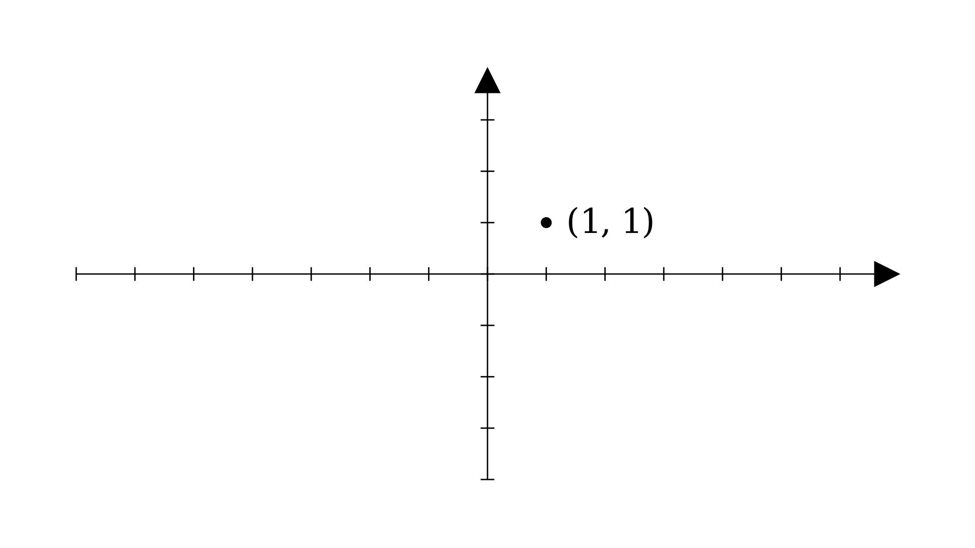
But that’s half the story. Vectors are defined to have both magnitude and direction. You can visualize it like this:
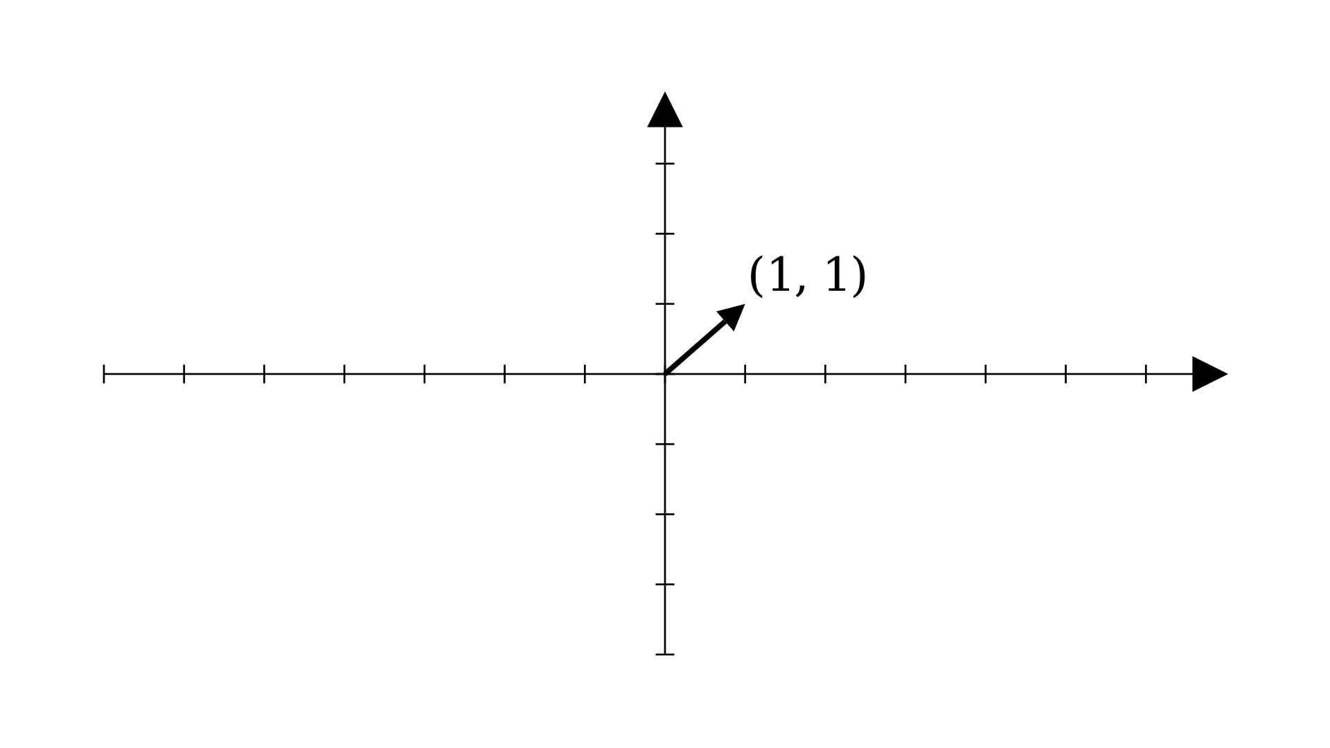
We looked at a 2-dimensional example. But vectors can be generalized to any number of dimensions that you require. What’s great about this is that all the operations we define work on vectors of any size. This means we can work with vectors in any \(n\) dimensional space (\(n\in\mathbb{N}\)) using the same principles and operations.
The beauty in this is that we can work with spaces that are greater (dimensionally) than what we can perceive (which is 3, we can perceive height, width, and depth). That is incredibly powerful, as we will see when we start with deep learning.
Magnitude?
In the previous section, I mentioned that all vectors have a magnitude and a direction. The direction part was pretty clear from the arrow visualization, let’s talk about the magnitude a little now (we’ll cover this in more detail when we talk about norms later)
You can think of magnitude as a measure of the “size” of the vector. Another intuition is how far the vector will take us if we travel from its tail to the tip of its arrow. Let’s find out how to calculate the magnitude if we consider the second intuition.
(I hope you know about Pythagoras’ Theorem)
Consider this diagram (I’ve added some labels to it):
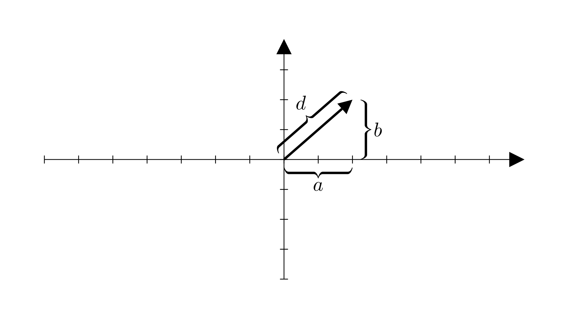
\(d\) is what we’re interested in, and we have \(a\) and \(b\). According to Pythagoras’ theorem:
\[d^2=a^2+b^2\]
And it’s trivial to deduce the rest from here:
\[d=\sqrt{a^2+b^2}\]
Here, \(d\) gives the magnitude of a vector in a 2-dimensional plane. But, we can generalize this formula to any number of dimensions like so:
\[d=\sqrt{a_1^2+a_2^2+…\ +a_n^2}\]
where \(a_i\) is an element of the vector \(a\).
A vector with unit magnitude has its \(d=1\).
Addition and multiplication
Addition of vectors is easy. Add the corresponding components together (components refer to the basis vectors, we talk about them in the next section). For example, consider \(\boldsymbol{u}=[1,\ 1]\) and \(\boldsymbol{v}=[2,\ 3]\). Then \(\boldsymbol{u}+\boldsymbol{v}\) will be:
\[ \begin{bmatrix} 1 \\ 1\end{bmatrix} + \begin{bmatrix} 2 \\ -2\end{bmatrix} = \begin{bmatrix} 3 \\ -1\end{bmatrix} \]
Addition of two vectors is the net result of moving along them. Here’s how you visualize it:
Multiplication of a vector with a scalar is even easier, multiply all entries with the number. For example, \(\boldsymbol{u}\) from the previous example when multiplied by 3 would be:
\[ 3\begin{bmatrix}1\\1\end{bmatrix}=\begin{bmatrix}3\times1\\3\times1\end{bmatrix}=\begin{bmatrix}3\\3\end{bmatrix} \]
Here’s what it looks like:
The \(\boldsymbol{\hat{i}}\) and \(\boldsymbol{\hat{j}}\) notation
Here’s a regular 2D graph, I’ve labeled it:
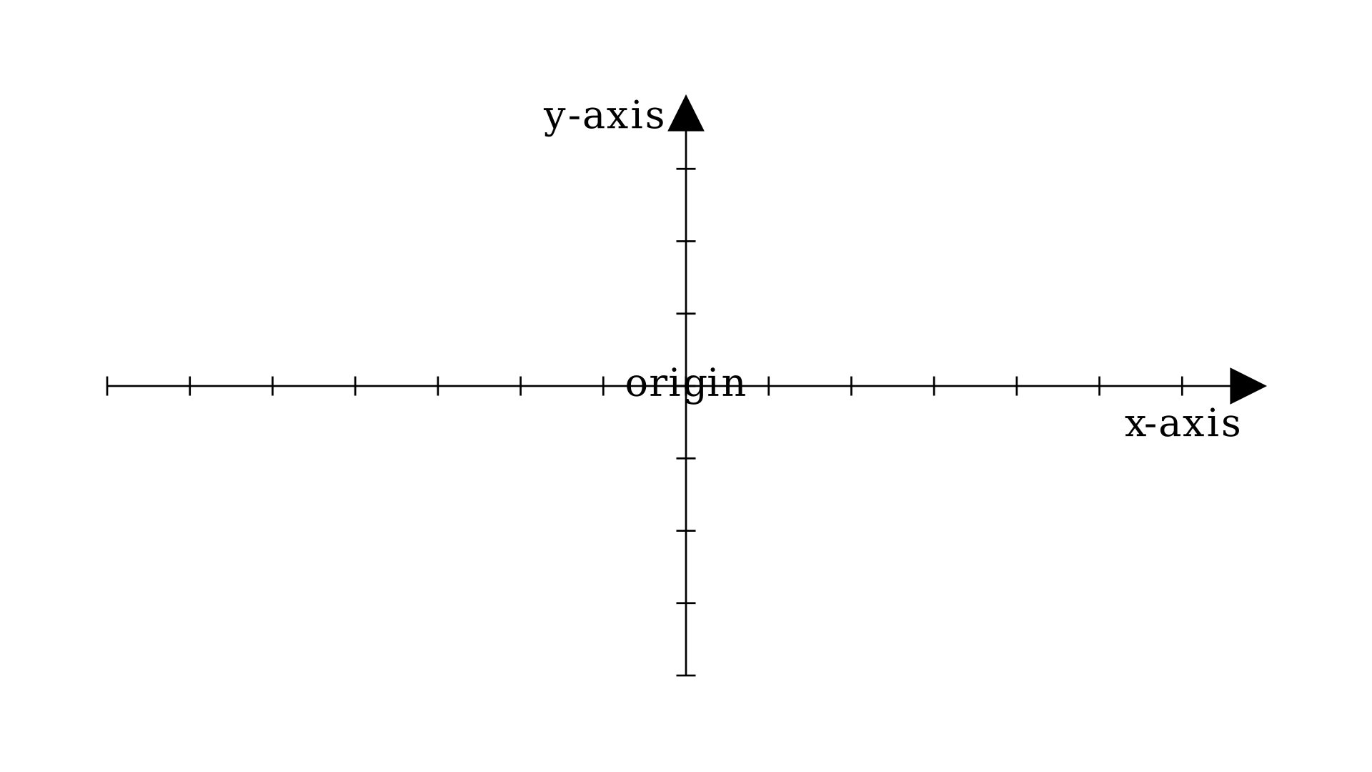
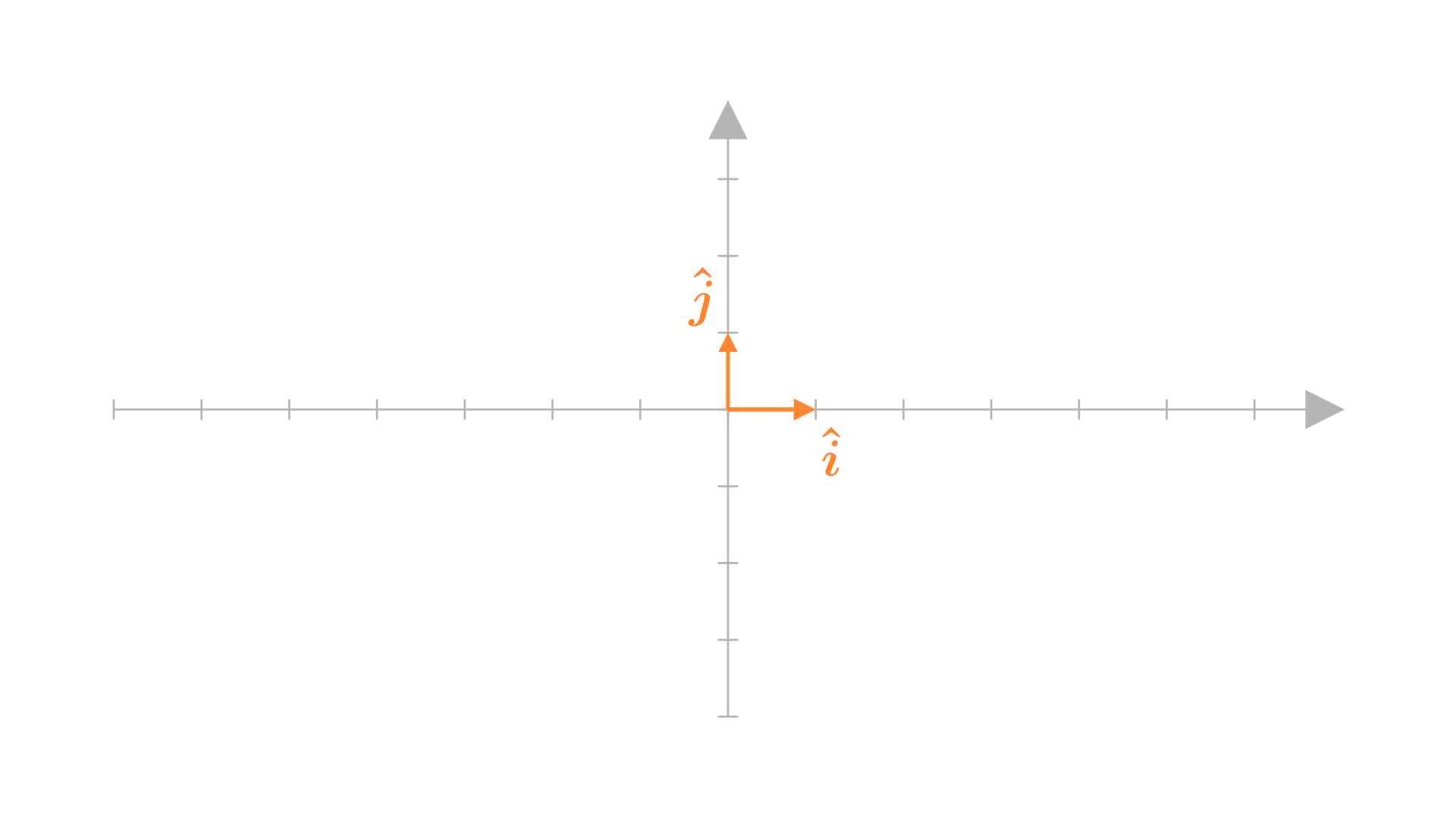
Let’s talk about the x and y axes. From what I can see they’ve got arrows. Does this mean that they’re vectors? Yes (not exactly, but we’ll assume they are for now), and there’s a special name for them. They’re called basis vectors. Why? Because they are the basis for all the points that we define in this 2D graph.
Consider this example we saw at the start:

Now let’s think about what this (1,1) means for a second. You probably know that it means this point lies 1 unit from the origin on the x-axis and 1 unit from the origin on the y-axis. Simple, right?
Now consider a vector \(\boldsymbol{a}=[2,\ 3]\)
Here’s another way to write it: \(\boldsymbol{a}=2\hat{i}+3\hat{j}\)
Looks familiar? That’s because it is. It means the same as 2 units from the origin on the x-axis and 3 units from the origin on the y-axis. It’s a different way to write it. But this right here gives us two important definitions: \(\hat{i}\) and \(\hat{j}\), which represent the vectors along the x and y axes respectively.
In fact, \(\hat{i}\) and \(\hat{j}\) are the basis vectors that we talked about thirty seconds ago. Their values for the above example are: \(\boldsymbol{\hat{i}}=[1,\ 0], \boldsymbol{\hat{j}}=[0,\ 1]\)
Thinking in terms of vectors
Now that we are aware of \(\hat{i}\) and \(\hat{j}\) as independent vectors, we can discuss about what the representation \(\boldsymbol{a}=2\hat{i}+3\hat{j}\) means in terms of basis vectors. The term \(2\hat{i}\) here means that \(\hat{i}\) is scaled by a factor of two. Same with \(3\hat{j}\). And the vector \(\boldsymbol{a}\) is the net result of moving along \(2\hat{i}\) and \(3\hat{j}\).
The implication we get from this is important: You can obtain any vector by multiplying the basis vectors by some scalar and adding them (not the complete truth. We discuss why in a later chapter where I talk about span).
That sounds trivial at first but think about it. This property will hold regardless of which basis vectors we pick. We could pick \(\boldsymbol{u}=[0.72,\ 1.234]\) and \(\boldsymbol{v}=[-1.2,\ 3.5]\) as the basis vectors, and we would still be able to obtain any point we want on the entire graph by multiplying them by some scalars and adding them.
BTW: This multiplication of a set of vectors by some scalars and adding them together is called a linear combination of those vectors.
That’s enough about vectors for now. Let’s talk about the elephant in the room.
Matrix
The reason I shoveled the basics of vectors in your face multiple times is so you understand what I am about to tell you now.
Carrying forward the computer science context, a matrix is a 2D array of scalars. Here’s what a matrix looks like: \(\boldsymbol{A}=\begin{bmatrix}1 & 2 \\ 3 & 4 \end{bmatrix}\)
Now the question nobody answered in school: What is a matrix though? What does it represent and why does it exist?
The answer: A matrix represents a function that transforms one vector space into another.
Wait, what?
Transformation of what?
Transforming a vector is exactly what it sounds like, changing one vector into another. But what do I mean when I say vector space?
A vector space means the “coordinate system” the vector lives in.
For example: \(\boldsymbol{a}=[1,\ 1]\) lives in the vector space defined by the basis vectors \(\hat{i}\) and \(\hat{j}\). Every single point in \(\boldsymbol{a}\)’s world is made up of some linear combination of \(\hat{i}\) and \(\hat{j}\). Similarly, \(\boldsymbol{b}=[1,1]\) lives in the vector space defined by the basis vectors \(\boldsymbol{u}=[0.75, 1.2]\) and \(\boldsymbol{v}=[-1, 0.5]\). But it is not the same vector as \(\boldsymbol{a}\) despite the same coordinates.
It’s like an example of relative motion, where a cup inside a train you travel in might appear stationary to you, but it moves at the same speed as the train for an observer outside the train.
Here’s what it looks like:
But then why do we transform one vector space into another? We just want one vector to turn into another vector, right? That’s because we are usually required to transform multiple vectors into their transformed counterparts and we need a solution applicable to all the possible input vectors. So, we define it generally and make a function out of it. This function is a mapping between a vector and what it should be when we transform it.
The intuition
Alright then, quick recap. Matrices are functions that transform one vector into another one. But how? How is a 2x2 grid of numbers supposed to be a function? Here’s where the basis vectors come into play. Remember what I told you about basis vectors around 5 minutes ago?

So here’s the idea: To define any vector in the vector space you only need the basis vectors because we can derive every point in that vector space by trying different linear combinations of those basis vectors.
So how do we describe a new vector space then?
By its basis vectors.
Armed with this new knowledge, you will now look at what’s inside a matrix:

To define a transformation, we only need to know where the basis vectors land after the transformation, the coordinates of which, are represented by a matrix. This implies that fundamentally, a matrix is a set of basis vectors of the transformed vector space.
Matrix multiplication
What’s matrix multiplication got anything to do with this? The answer to that is matrix multiplication is the operation we use to transform vectors.
To understand what that meant, let’s look at what happens when we multiply a matrix with a vector. Consider this example:
\[\begin{bmatrix}1 & 3 \\ 2 & -1\end{bmatrix}\begin{bmatrix}2 \\ 1\end{bmatrix}\]
Easy enough, right? Multiply the row elements of the matrix to the respective column elements of the vector, add the corresponding row-column element products and you have your answer:
\[\begin{bmatrix}1 & 3 \\ 2 & -1\end{bmatrix}\begin{bmatrix}2 \\ 1\end{bmatrix}=\begin{bmatrix}1\times2+3\times1 \\ 2\times2+(-1)\times1\end{bmatrix}=\begin{bmatrix}5 \\ 3\end{bmatrix}\]
But, if you pay close attention to the actual multiplication action between the square brackets, an interesting pattern emerges:
\[\begin{bmatrix}1 & 3 \\ 2 & -1\end{bmatrix}\begin{bmatrix}2 \\ 1\end{bmatrix}= \overbrace{2\begin{bmatrix}1 \\ 2 \end{bmatrix} + 1\begin{bmatrix} 3 \\ -1 \end{bmatrix}}^{\text{the intuition}} = \\ \begin{bmatrix}1\times2 \\ 2\times2 \end{bmatrix}+ \begin{bmatrix}3\times1 \\ -1\times1 \end{bmatrix} = \underbrace{\begin{bmatrix}1\times2 + 3\times1 \\ 2\times2 + (-1)\times1 \end{bmatrix}}_{\text{what we were taught}} = \begin{bmatrix}5 \\ 3 \end{bmatrix}\]
Okay so remember what I told you about matrices in the previous section? A set of basis vectors, right? Let’s name these basis vectors for brevity. Let \(\boldsymbol{u}=[1,\ 2]\) and \(\boldsymbol{v}=[3,\ -1]\). What does the above multiplication look like now?
\[\begin{bmatrix}1 & 3 \\ 2 & -1\end{bmatrix}\begin{bmatrix}2 \\ 1\end{bmatrix}=2\begin{bmatrix}1 \\ 2\end{bmatrix}+1\begin{bmatrix}3 \\ -1\end{bmatrix}=2\boldsymbol{u}+\boldsymbol{v}\]
Notice anything familiar? If you guessed it looks like \(2\boldsymbol{\hat{i}}+\boldsymbol{\hat{j}}\) then you guessed correct. So what does this mean? It means multiplication of a vector by a matrix is that vector, but in a vector space described by some other basis vectors.
Remember how I told you \(\hat{i}=[1,\ 0]\) and \(\hat{j}=[0,\ 1]\)?
\[\overbrace{\begin{bmatrix}1 & 0 \\ 0 & 1\end{bmatrix}}^{\hat{i}\text{ and }\hat{j}}\begin{bmatrix}2\\3\end{bmatrix}=\begin{bmatrix}2\\3\end{bmatrix}\]
We don’t mention it like this because it would be a hassle. And also because the matrix is an identity matrix (more on identity matrices in the upcoming chapters).
So in a nutshell, what multiplying a vector by a matrix does is, it gives you the coordinates of the vector but on the coordinate system of some different basis vectors, in terms of the default coordinate system we’re using.
If the second half of last sentence confused you, it means the result we obtain is in terms of the default \(\hat{i}\) and \(\hat{j}\) coordinate system. Because in terms of the new basis vectors, the coordinates remain the same, i.e. \([2,\ 1]\). Notice how its still \(2\boldsymbol{u}+\boldsymbol{v}\), but the value on the default system becomes \(5\hat{i}+3\hat{j}\)?
(P.S. These values of \(\hat{i}\) and \(\hat{j}\) are almost always the same, unless specified otherwise)
Phew
That was a lot to take in. This is why I have split this one post into two. Next time, we will cover more topics about matrices, and take a quick look at tensors.
Another thing worth a mention is that I’ve only taken examples of 2x2 matrices, and vectors in 2-dimensions. The reason is ease in explanation and understanding. In practice, we work with much bigger vectors and matrices, and its important to understand what’s going on instead of rushing in blindly.
Reality check
If you understood what you read, you should be able to answer the following questions satisfactorily (to whose satisfaction you ask? Yours of course!)
- What is a scalar?
- What is a vector?
- What do you mean by the magnitude of a vector?
- How do you add two vectors?
- What does the addition of vectors signify?
- How do you multiply a scalar to a vector?
- What are basis vectors?
- What is a matrix?
- How does a matrix transform a vector space?
Extra references
3Blue1Brown’s Essence of linear algebra series was a huge help in gaining the intuition I’ve provided. You should definitely check it out.
Thanks for reading to the end. See you next time.